Graph Attention Multi-Layer Perceptron
Motivation
The size of the K-hop neighbors grows exponentially to the number of GNN layers (High Memory Cost).
GNN has to read great amount of data of neighboring nodes to compute the single target node representation, leading to high communication cost in a distributed environment (High Communication Cost).
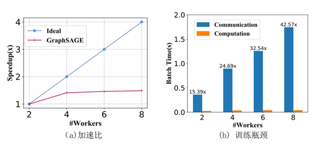
GNN的每一次特征传播都需要拉取邻居特征,对于k层的GNN来说,每个节点需要拉取的k跳以内邻居节点特征随着层数增加以指数增加,会占用大量内存。对于稠密的连通图,每个节点在每次训练的时候几乎需要拉取全图的节点信息,造成海量的通信开销。
A commonly used approach to tackle the issues is sampling.
- The sampling quality highly influences the model performance, and it still needs communication in each step (reduce neighbors ).
Sampling的方法虽然可以减少邻居数量,减轻内存压力,但是仍要消息传递。
Some method (e.g., SGC) decouples the feature propagation and the non-linear transformation process.
The feature propagation is executed during pre-processing.
Only the nodes of training set get involved in the model training.
The decoupling methods are more suitable for distributed training.
现有方法分离消息传递和非线性变化,提取收集好特征,后期直接用全连接变化即可。
Challenges
- The decoupling methods adopting fixed layers of feature propagation, leading to a fixed RF of nodes.
- The local information and long-range dependencies cannot be fully leveraged at the same time.
- This makes them lack the flexibility to model the interesting correlations on node features under different reception fields.
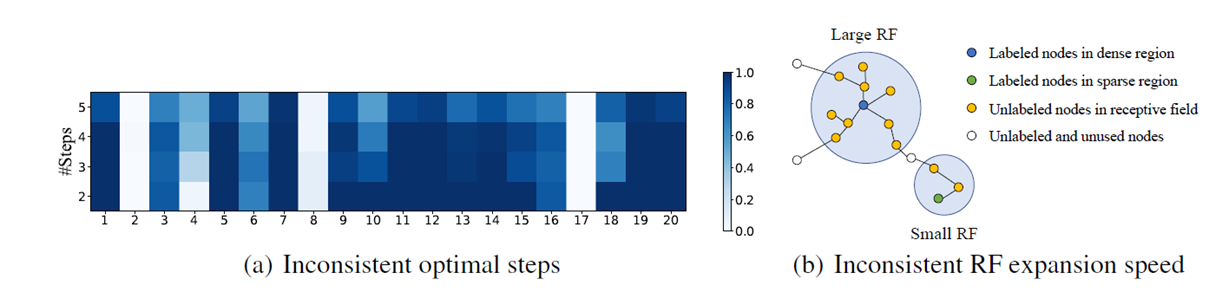
我们通过一个简单的示例来说明这个问题。图4中有1个被标蓝的节点并位于图中相对稠密的区域,而绿色节点位于图中相对稀疏的区域。同样进行2次特征传播操作,可以看到位于稠密区域的蓝色节点的感受野已经相对较大了,而位于稀疏区域的绿色节点的感受野却只包含了3个节点。这个实例形象地说明了不同节点的感受野的扩张速度存在较大的差异。在GNN中,一个节点感受野的大小表示它能捕获邻域信息的多少,感受野太大,则该节点可能会捕获许多不相关节点的信息,感受野太小,则该节点无法捕获足够的邻域信息得到高质量的节点表示。因此,对于不同特征传播步数的节点特征,GNN模型需要对不同的节点自适应地分配权重。否则,便会出现无法兼顾位于稠密区域和稀疏区域节点的情况,导致最后无法得到高质量的节点表示。
Contribution
- Propose a decoupling methods method that can be applied in huge graph and distributed environment.
- Propose three node-adaptive graph learning mechanisms to meet the requires of different nodes with different propagation steps.
- Achieve the STOA performance in the three largest graph benchmarks while maintains high scalability and efficiency.
Preliminaries
Graph-wise Propagation
- Recently studies have observed that non-linear feature transformation contributes little to the performance of the GNNs as compared to feature propagation.
- They reduces GNNs into a linear model operating on K-layers propagated features.
Graph-wise propagation和之前我们介绍的node-wise propagation 的先传播再非线性变化不一样,是直接得到一个K跳内的邻接的邻接矩阵和$\hat{A}^K$,然后一次性计算传播结果,提前收集好K-hop特征$X^K$,然后直接用全连接之类的变化即可。
显然在训练过程中不需要消息传递,结点K-hop特征直接被当成特征输入网络即可。
Layer-wise Propagation
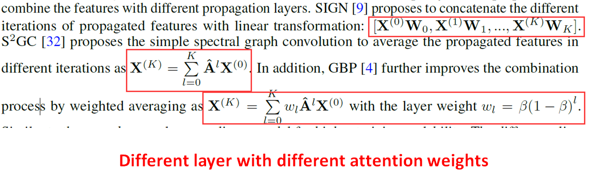
Following SGC, some recent methods adopt layer-wise propagation combining the features with different propagation layers.
The GAMLP Model
GAMLP decomposes the end-to-end GNN training into three parts: feature propagation, feature combination with RF attention, and the MLP training.
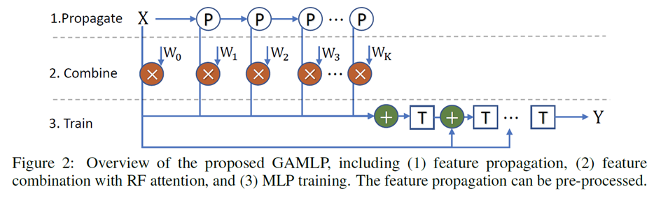
As the feature propagation is pre-processed only once, and MLP training is efficient and salable, we can easily scale GAMLP to large graphs. Besides, with the RF attention, each node in GAMLP can adaptively get the suitable
Feature Propagation
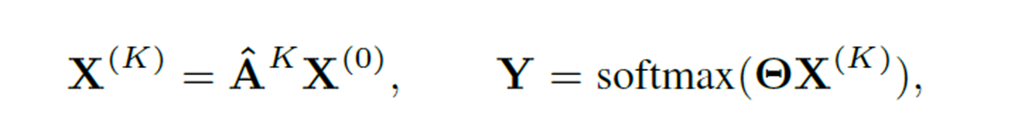
Parameter-free K-step feature propagation as:
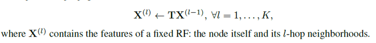
After K-step feature propagation, we correspondingly get a list of propagated features under different propagation steps:
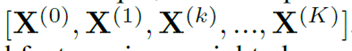
Average these propagated features in a weighted manner
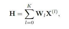
Receptive Field Attention
Get the attention weight $W_l$ for different layers.
Smoothing Attention
Suppose we execute feature propagation for infinite times. In that case, the node embedding within the same connected component will reach a stationary state (Over smoothing).
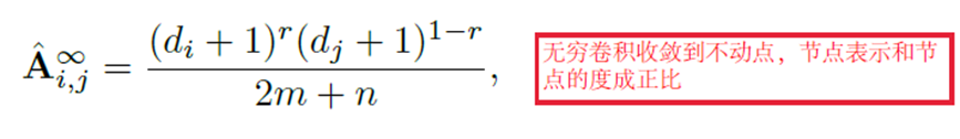

平滑注意力机制(Smoothing):把经无穷次传播的节点特征作为参考向量。在实际计算的时候有公式可以直接带入数值求解,并不需要真的进行无穷次特征传播。该注意力机制希望能够学习到不同传播步数的节点特征相对于的距离,并用这个距离来指导权重的选择。
Recursive Attention
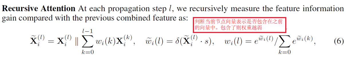
递归注意力机制(Recursive):使用递归计算的方式,在计算赋予经L步传播的节点特征 的权重时,把前 L-1步的融合节点特征作为参考向量。该注意力机制希望能够学习到 $X^L$相比前L-1步的融合节点特征的信息增益,并用这个信息增益来指导权重的选择。
JK Attention
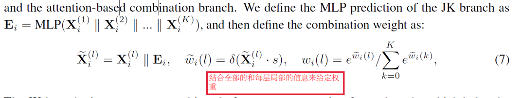
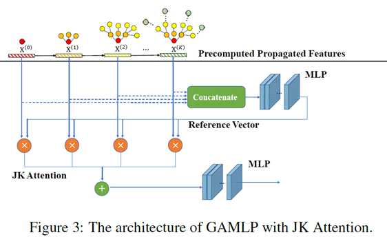
知识跳跃注意力机制(JK):如图7所示,把预处理阶段得到的所有经特征传播的节点特征全都按列拼接起来,并让这个向量过一个MLP,以MLP的输出结果作为参考向量。该注意力机制中的参考向量包含了所有K个经特征传播的节点特征矩阵中的信息,该注意力机制希望能够学习到不同传播步数的节点特征相对于大向量 的重要性,并用这个重要性来指导权重的选择。(可以理解为是一个局部的over smoothing attention).
Model Training
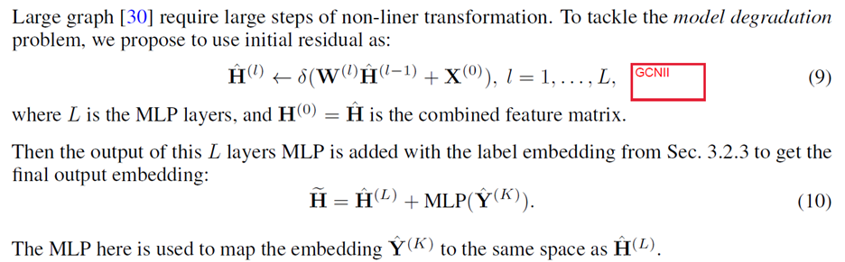
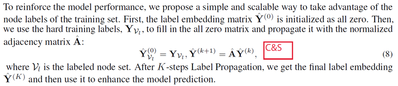
Incorporating Label Propagation
Reliable Label Utilization (RLU)
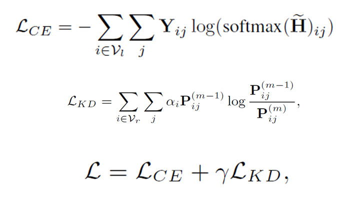
To better utilize the predicted soft label (i.e., softmax outputs), we split the whole training process into multiple stages, each containing a full training procedure of the GAMLP model.
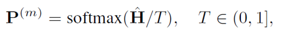
Here, we denote the prediction results of m-th stage as:
we adopt the predicted results for the nodes in the validation set and the test set at the last stage to enhance the label propagation.
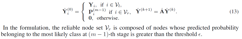
增加label propagation的初始数量,把上次训练得到的高可信度的结点标签也作为真实标签加入,T controls the softness of the softmax distribution
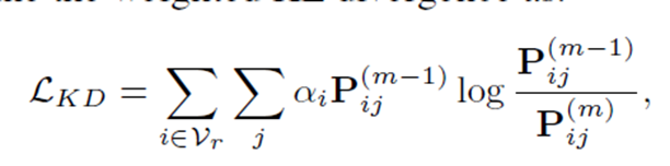
Reliable Label Distillation
To fully take advantage of the helpful information of the last stage, we also included a knowledge distillation module in our model. we only include the nodes in the reliable node set $𝑉_r$ at (m-1)-th
stage (m > 1) and then define the weighted KL divergence as:
Loss
Experiments
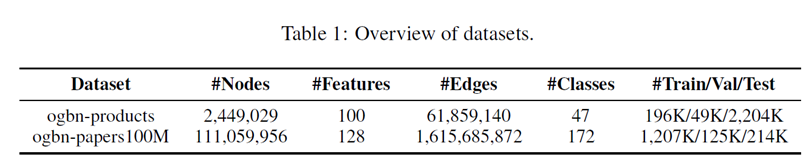
Datasets
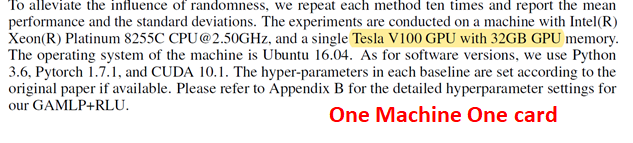
Implementation
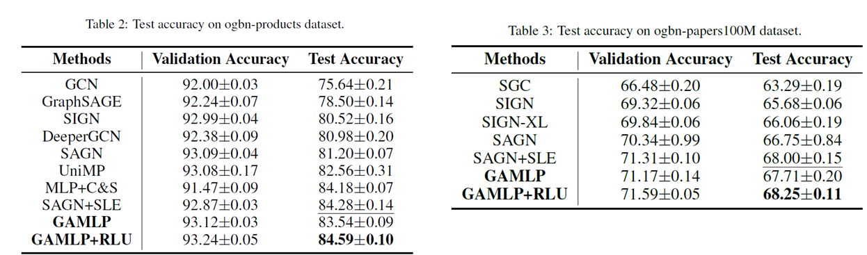
Results
单机单卡跑10亿级别结点,在Ogb拿到了全球第一。
The weights of propagated features with larger steps drop faster as the degree grows, which indicates that our attention mechanism could prevent high-degree nodes from including excessive irrelevant nodes which lead to over-smoothing.
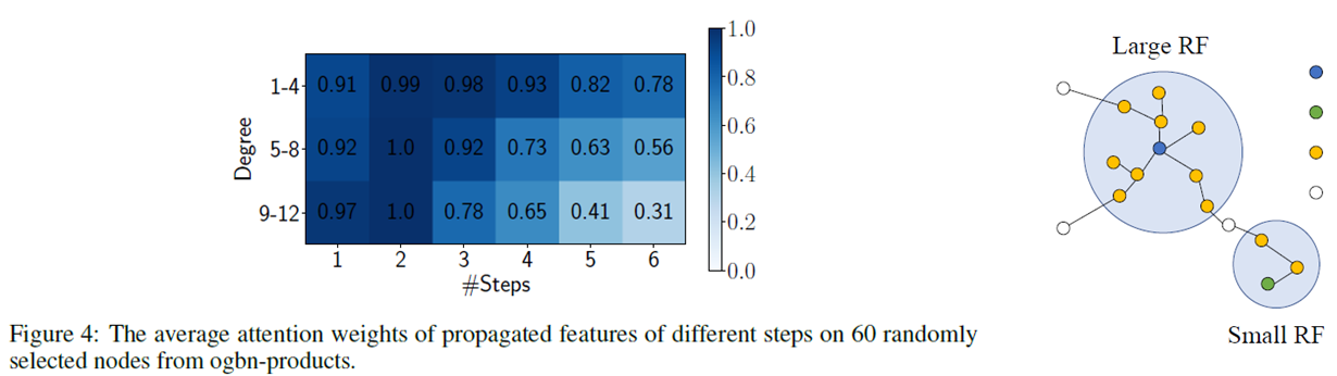
度数越高越dense,因此自然用的是局部的信息。
Conclusion
- This paper proposed many tricks (i.e., attention, GCNII, label propagation, knowledge distillation) that can be used in our method to boost the performance in the final stage.
- The decoupling and weighted average methods can be extended to solve the huge HIN case (e.g., knowledge graph).