Motivation
TL;DR: The major motivation behind this method is: they use Jackknife to estimate the distribution of error, then it use a threshold to find the upper- and lower-bound of the error in the distribution, which is used for quantifying the uncertainty.
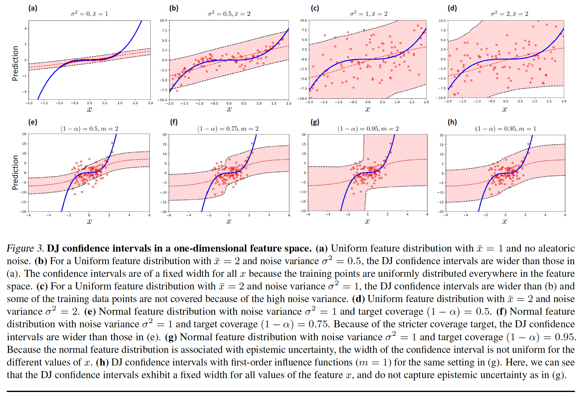
Quantifying the uncertainty over the predictions of existing deep learning models remains a challenging problem.
Deep learning models are increasingly popular in various application domains. A key question often asked of such model is “Can we trust this particular model prediction?” This is highly relevant applications wherein predictions are used to inform critical decision-making.
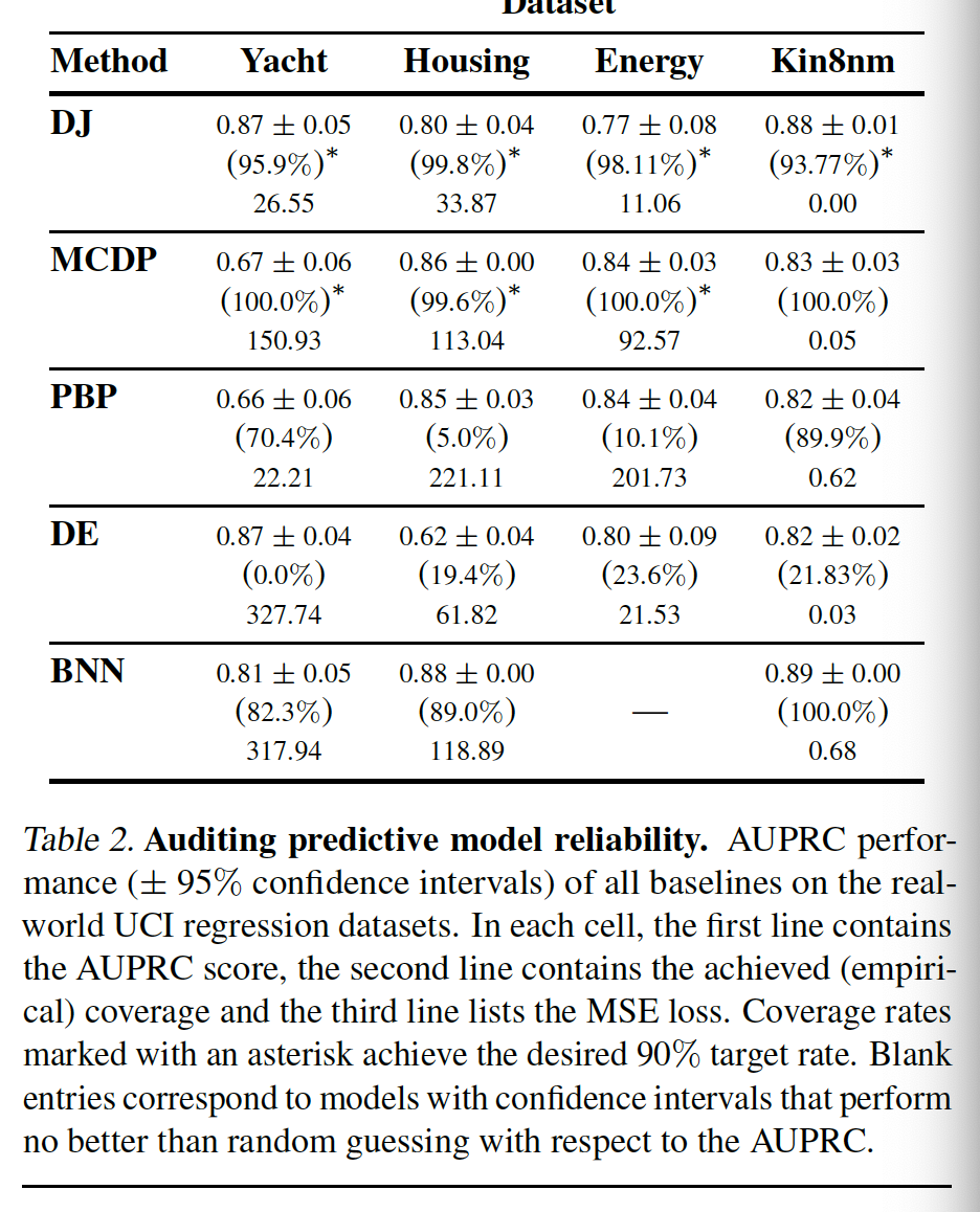
Existing methods for uncertainty estimation are based on Bayesian neural network. They do not guarantee (1) cover the true prediction targets with high probability (2) discriminate between high- and low-confidence prediction.
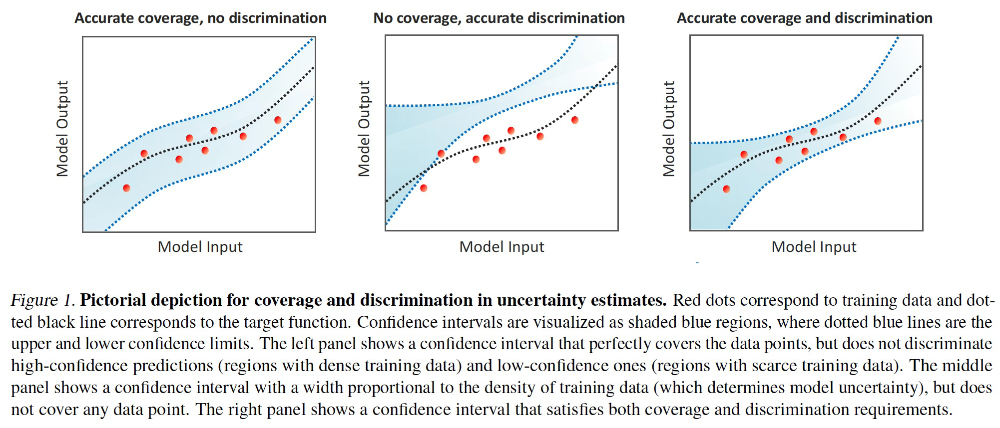
Frequentist coverage: denotes whether the estimated confidence interval cover the data points.
Discrimination: denotes whether the model is able to discriminate
high-confidence predictions (regions with dense training data) and low-confidence ones (regions with scarce training data).
Existing methods for uncertainty estimation are based predominantly on Bayesian neural networks.
- Bayesian neural networks require significant modifications to the training procedure.
- Approximate the posterior distributions could jeopardize both the coverage and discrimination performance of the resulting credible intervals.
Contributions
Propose the discriminative jackknife (DJ) to estimate the uncertainty over samples inspired by the jackknife leave-one-out (LOO) re-sampling procedure
To avoid exhaustively re-training the model for each sample, they adopt the high-order influence function to approximate the impact of each sample.
DJ is post-hoc to the model training. It is capable of improving coverage and discrimination without any modifications to the underlying predictive model.
Preliminaries
Learning setup
Considering a standard supervised learning setup, we try to minimize the prediction loss on the training data $\mathcal{D}n = {(x_i, y_i)}{i=1}^n$.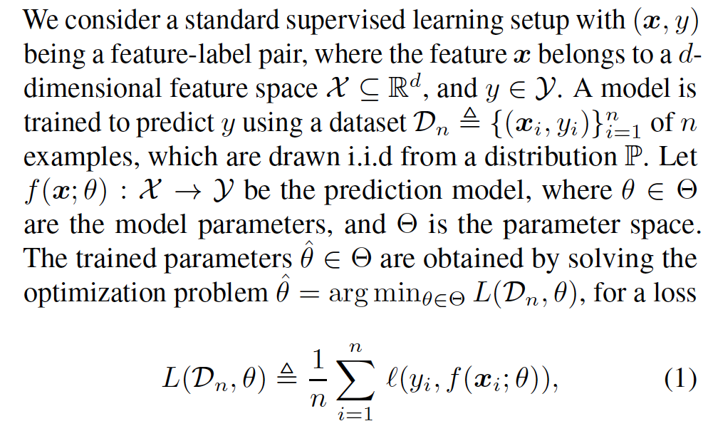
Uncertainty Quantification
We aim to estimate the uncertainty in the model’s prediction though the pointwise confidence interval $\mathcal{C}(x;\hat{\theta})$.
The degree of uncertainty in the model’s prediction is quantified by the interval width
Frequentist coverage
This is satisfied if the confidence interval $\mathcal{C}(x;\hat{\theta})$ covers the true target $y$ with a prespecified coverage probability of $(1-\alpha), \alpha \in (0,1)$.
discrimination
The confidence interval is wider for test points with less accurate predictions.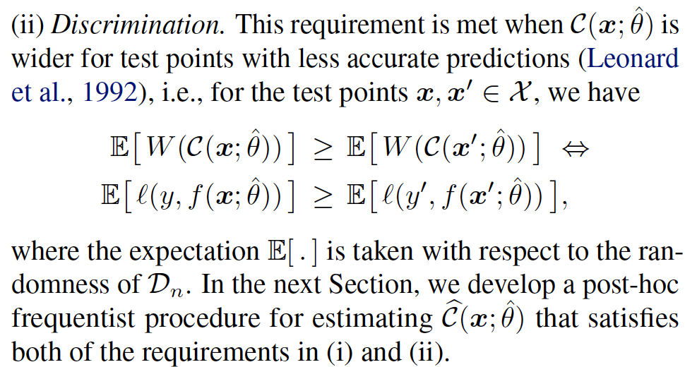
Discriminative Jackknife
Classical Jackknife
The jackknife quantifies predictive uncertainty in terms of the average prediction error, which is estimated via leave-one-out (LOO) construction found by systematically leaving out each sample in $\mathcal{D}_n$, and evaluating the error of the restrained model on the left-out samples.
For a target coverage of $(1-\alpha)$, the native jackknife is
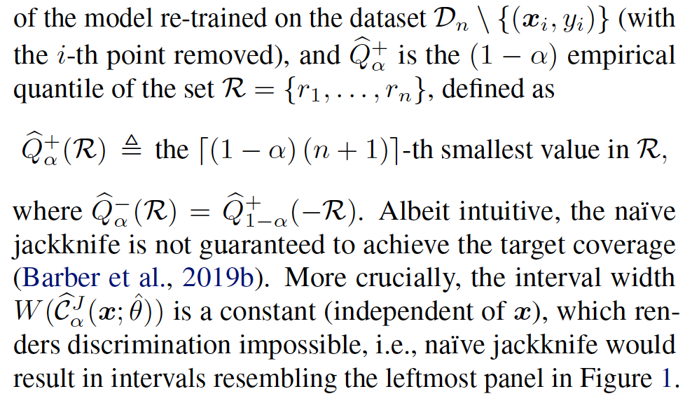
$\mathcal{\hat Q}_\alpha^+(\mathcal{R})$: $(1-\alpha)(n+1)$-th smallest element of $\mathcal{R}$.
The interval width is constant, which renders discrimination impossible.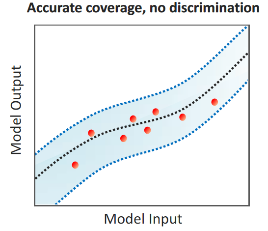
DJ Confidence Intervals
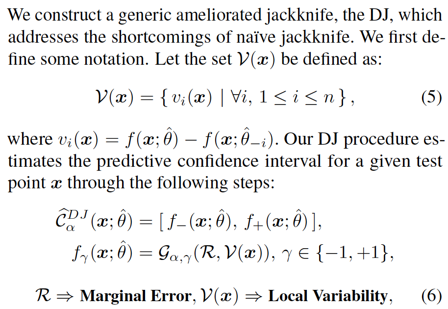
The $\mathcal{G}_{\alpha,\gamma}$ is a quantile function applied on the elements of the sets of marginal prediction errors $\mathcal{R}$ and local prediction variability $\mathcal{V}$.
The prediction error is constant, i.e., does not depend on $x$, hence it only contributes to coverage but does not contribute to discrimination.
The local variability term depends on $x$, hence it fully determines the discrimination performance.
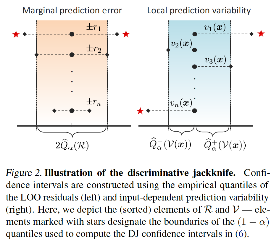
The confidence interval is bounded by
Efficient Implementation via Influence Functions

Approximate the $\hat\theta_i$ using the high-order influence function.
Influence functions enable efficient computation of the effect of a training data point $(x_i,y_i)$ on $\hat\theta$. This is achieved by evaluating the change in $\hat\theta$, if $(x_i,y_i)$ was up-weighted by a small factor $\epsilon$.


Removing a training point is equivalent to upweighting it by $\frac{-1}{n}$.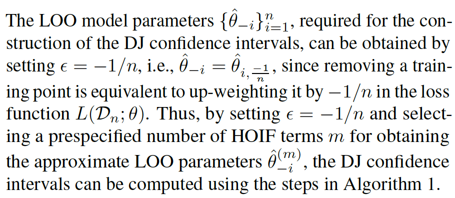

Experiments
